什么有效区域？

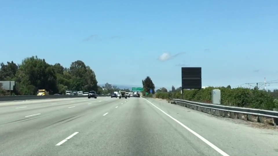
设想自动驾驶的摄像头固定在车辆前端，拍摄到的图像是固定大小的，例如：960*540；但是感兴趣的车道线不是分布在整个图像中的，而是正前方一小段区域。如果为了提取车道线，对整个图像都进行处理，一是加剧了计算单元的负担，二是没有任何收益。所以我们要让计算机只处理“有效的区域”

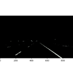
摄像头拍到的图像

真正感兴趣的区域

图像基础-图像的坐标

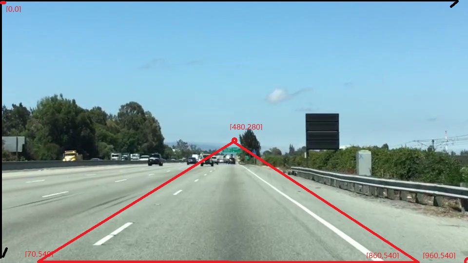
计算机存储的图像的坐标轴与我们认知中的常见的xy坐标有些差异。在计算机中以图像左上角为原始坐标[0,0],x方向为横向，y方向为纵向。转换为数组之后与数组下标相吻合，这是我们在处理计算机图像过程中首先需要注意的。

图像中的坐标系

选定区域范围

根据这个坐标，我们选定我们的感兴趣范围为一个三角形，三个顶点分别为：
左下角：[70,540]
右下角：[860,540]
上顶点：[480, 280]
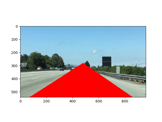
也就是文章开头图像中的红色三角形区域，下面我们用代码将该区域划出来。

测试代码：

import matplotlib.pyplot as plt
import matplotlib.image as mpimg
import numpy as np
from PIL import Image
from numpy import array

# Read in the image and print out some stats
# image = mpimg.imread('ColorSelectionTest.png')
image_P = Image.open('ColorSelectionTest.jpg')
print('This image is: ',type(image_P), 
         'with dimensions:', image_P.size)

image=array(image_P)

# Pull out the x and y sizes and make a copy of the image
ysize = image.shape[0]
xsize = image.shape[1]
region_select = np.copy(image)

left_bottom = [70,540]
right_bottom = [860,540]
apex = [480, 280]

# Fit lines (y=Ax+B) to identify the  3 sided region of interest
# np.polyfit() returns the coefficients [A, B] of the fit
fit_left = np.polyfit((left_bottom[0], apex[0]), (left_bottom[1], apex[1]), 1)
fit_right = np.polyfit((right_bottom[0], apex[0]), (right_bottom[1], apex[1]), 1)
fit_bottom = np.polyfit((left_bottom[0], right_bottom[0]), (left_bottom[1], right_bottom[1]), 1)

# Find the region inside the lines
XX, YY = np.meshgrid(np.arange(0, xsize), np.arange(0, ysize))
region_thresholds = (YY > (XX*fit_left[0] + fit_left[1])) & \
                    (YY > (XX*fit_right[0] + fit_right[1])) & \
                    (YY < (XX*fit_bottom[0] + fit_bottom[1]))

# Color pixels red which are inside the region of interest
region_select[region_thresholds] = [255, 0, 0]
# print(region_thresholds)

# Display the image
plt.imshow(region_select)
plt.show()

测试结果

彩蛋：np.polyfit，np.meshgrid

meshgrid

meshgrid的官方说明

为什么要meshgrid

我们分解图像的区域是通过两点之间的连接线来进行分解的，连接线为直线，在坐标轴上可以通过方程表示：

首先我们想得到的是整个图像的坐标轴，即x，y矩阵，分别代表着x轴和y轴

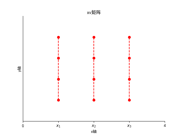
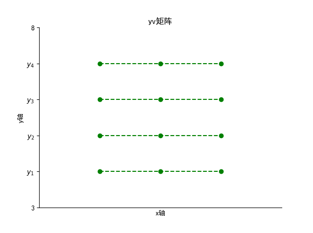
获取这个坐标轴矩阵的方法就是meshgrid

meshgrid的用法

xv,yv = meshgrid(x,y)
xv,yv = meshgrid(x)与xv,yv = meshgrid(x,x)是等同的
xv,yv,zv = meshgrid(x,y,z)生成三维数组，可用来计算三变量的函数和绘制三维立体图
上面的这些都是直接进行解包后的返回值。其实他返回的是一个list列表，列表中存放的xv,yv,zv的这些numpy数组。

import numpy as np

x = np.array([1,2,3]) #X_{x} = 3
y = np.array([4,5,6,7]) #X_{y} = 4

xv,yv = np.meshgrid( x , y )

print(xv)
print(yv)

[[1 2 3]
 [1 2 3]
 [1 2 3]
 [1 2 3]]
[[4 4 4]
 [5 5 5]
 [6 6 6]
 [7 7 7]]

polyfit

polyfit官方链接

polyfit官方链接

为什么要polyfit

在meshgrid的章节我们讲过，直线的表示可以用y=ax+b表示，meshgrid解决了x/y，但a和b该如何得到呢？这就需要拟合函数，也就是polyfit函数了。这是一个非常强大的函数，可以拟合各种多项式，在现在这个场景中我们只需要拟合直线，也就是一次多项式

如何使用polyfit

fit_left = np.polyfit((left_bottom[0], apex[0]), (left_bottom[1], apex[1]), 1)

传入参数分别为两个点坐标，以及最后的1表示一次多项式，返回的是一个有两个参数的一维数组，分别表示a和b。

以下代码会加深大家的了解，请在jupyter中运行并调整参数

import numpy as np
from matplotlib import pyplot as plt

def linear_regression(x,y):
    #y=bx+a，线性回归
    num=len(x)
    b=(np.sum(x*y)-num*np.mean(x)*np.mean(y))/(np.sum(x*x)-num*np.mean(x)**2)
    a=np.mean(y)-b*np.mean(x)
    return np.array([b,a])
def f(x):
    return 2*x+1
x=np.linspace(-5,5)
y=f(x)+np.random.randn(len(x))#加入噪音
y_fit=np.polyfit(x,y,1)#一次多项式拟合，也就是线性回归
print(linear_regression(x,y))
print(y_fit)
plt.plot(x,f(x),'r',label='original')
plt.scatter(x,y,c='g',label='before_fitting')#散点图
plt.plot(x,x*y_fit[0]+y_fit[1],'b--',label='fitting')#通过polyfit获取的直线
plt.title('polyfitting')
plt.xlabel('x')
plt.ylabel('y')
plt.legend()#显示标签
plt.show()

测试结果

代码链接

github for Zhaoweiwei