
04-01 Deep_Neural_Network–在TensorFlow中建立深度神经网络
之前我们已经通过TensorFlow建立了自己的分类器,现在我们将从基本的分类器转变为深度神经网络。我们以识别MNIST数据集中的手写数字作为目标,通过代码一步步建立神经网络。
代码
from tensorflow.examples.tutorials.mnist import input_data
mnist = input_data.read_data_sets(".", one_hot=True, reshape=False)
#MNIST数据集已经可以用one-hot编码的形式提供
import tensorflow as tf
# 学习的参数大家可以自行调节
learning_rate = 0.001
training_epochs = 20
batch_size = 128 # Decrease batch size if you don't have enough memory
display_step = 1
n_input = 784 # MNIST data input (img shape: 28*28)
n_classes = 10 # MNIST total classes (0-9 digits)
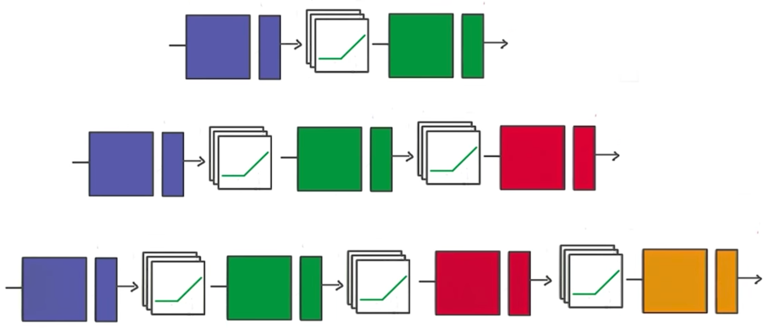
#隐藏层的数量也就是我们上一节中讲的ReLU的数量H,这个值也可以调节
n_hidden_layer = 256 # layer number of features
# 权重和偏置需要有两份,一份是wx+b;另一份是w1*ReLU输出+b1
weights = {
'hidden_layer': tf.Variable(tf.random_normal([n_input, n_hidden_layer])),
'out': tf.Variable(tf.random_normal([n_hidden_layer, n_classes]))
}
biases = {
'hidden_layer': tf.Variable(tf.random_normal([n_hidden_layer])),
'out': tf.Variable(tf.random_normal([n_classes]))
}
# tf Graph input
x = tf.placeholder("float", [None, 28, 28, 1])
y = tf.placeholder("float", [None, n_classes])
#由于输入的是28*28*1的图像,需要将它转变为784的一维数组输入
x_flat = tf.reshape(x, [-1, n_input])
#建立两层神经网络
# Hidden layer with RELU activation
layer_1 = tf.add(tf.matmul(x_flat, weights['hidden_layer']), biases['hidden_layer'])
layer_1 = tf.nn.relu(layer_1)
# Output layer with linear activation
logits = tf.matmul(layer_1, weights['out']) + biases['out']
#GradientDescentOptimizer在TensorFlow入门那一章节讲过
# Define loss and optimizer
cost = tf.reduce_mean(tf.nn.softmax_cross_entropy_with_logits(logits=logits, labels=y))
optimizer = tf.train.GradientDescentOptimizer(learning_rate=learning_rate).minimize(cost)
# Initializing the variables
init = tf.global_variables_initializer()
# Launch the graph
with tf.Session() as sess:
sess.run(init)
# Training cycle
for epoch in range(training_epochs):
total_batch = int(mnist.train.num_examples/batch_size)
# Loop over all batches
for i in range(total_batch):
#mnist.train.next_batch()每次返回一个训练集的子集
batch_x, batch_y = mnist.train.next_batch(batch_size)
# Run optimization op (backprop) and cost op (to get loss value)
sess.run(optimizer, feed_dict={x: batch_x, y: batch_y})
# Display logs per epoch step
if epoch % display_step == 0:
c = sess.run(cost, feed_dict={x: batch_x, y: batch_y})
print("Epoch:", '%04d' % (epoch+1), "cost=", \
"{:.9f}".format(c))
print("Optimization Finished!")
# Test model
correct_prediction = tf.equal(tf.argmax(logits, 1), tf.argmax(y, 1))
# Calculate accuracy
accuracy = tf.reduce_mean(tf.cast(correct_prediction, "float"))
# Decrease test_size if you don't have enough memory
test_size = 256
print("Accuracy:", accuracy.eval({x: mnist.test.images[:test_size], y: mnist.test.labels[:test_size]}))
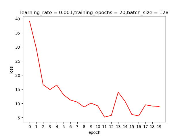
learning rate=0.001,epoch=20测试结果
learning rate=0.0001,epoch=20测试结果
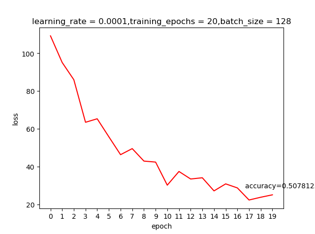
我们之前提到learning rate越大虽然学习越快,但精度可能并不好;上面这两个结果好像并不好解释,那是不是我们的学习回合不够多呢?那就把epoch加大到200看看有什么申请的反应
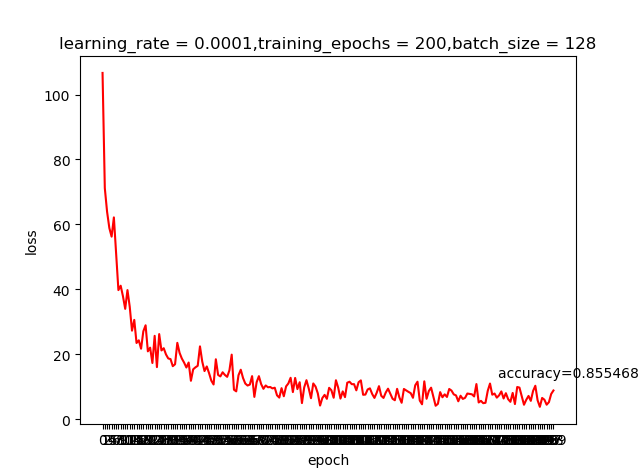
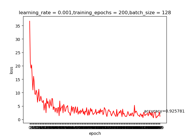
哈,这就是神经网络的神奇,调整一个小参数也会有很大的差别。感兴趣的同学可以把激活函数变成我们之前提到的sigmoid,看看有什么变化
发表评论
Want to join the discussion?Feel free to contribute!